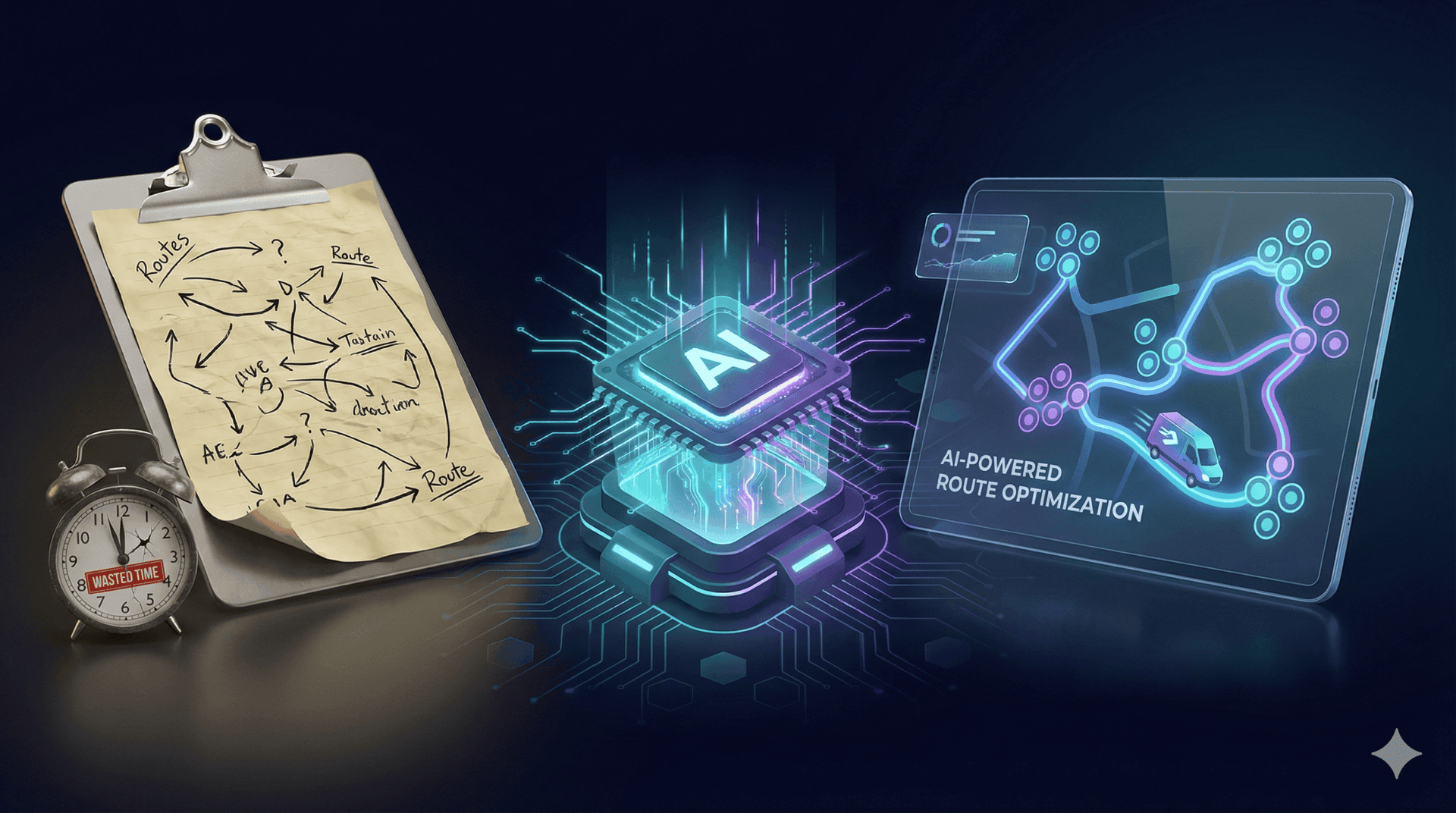
How AI Reduces Drive Time

The mechanics behind AI-optimized routing, and why manual dispatching can’t compete.

Your technicians spend 2-3 hours per day just driving. That’s 25-35% of their shift: unpaid, unproductive windshield time. For a 5-technician team, that’s 10-15 hours of lost productivity every single day.

AI fixes this by analyzing job locations, traffic patterns, and time windows to sequence jobs that eliminate backtracking, cluster nearby appointments, and adapt routes in real time.

Instead of a dispatcher manually assigning jobs based on availability alone, AI groups three jobs within a 2-mile radius for one technician while routing another to a different cluster.

New to AI routing? Start with how AI route optimization works.

This article breaks down the specific mechanisms, from geographic clustering to real-time traffic adaptation, that translate routing decisions into measurable time savings.

The Six Types of Wasted Drive Time AI Eliminates

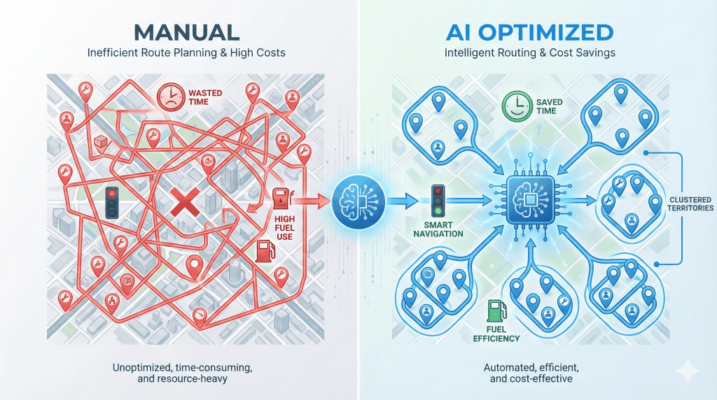
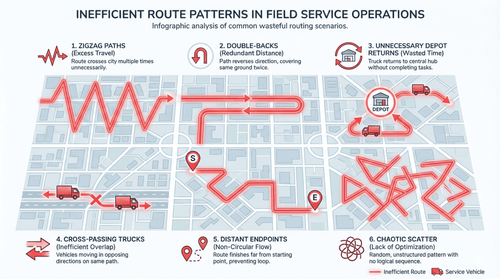
Manual dispatching creates six distinct patterns of wasted drive time that AI systematically eliminates.

1. Backtracking

Backtracking occurs when a technician travels back through previously covered territory to reach the next job, adding unnecessary miles and time to their route.

In manual dispatching, this often happens when jobs are assigned based on availability or urgency without considering geographic sequence.

A tech finishes a job up north, drives south for the next one, then back north again, same roads, twice.

2. Zone Ping-Ponging

This happens when technicians jump between service zones without a logical geographic flow.

A dispatcher assigns Job A in the northwest, Job B in the southeast, then Job C back in the northwest, creating a zigzag pattern across the metro area.

3. Depot Deadheading

Unnecessary returns to the depot mid-day for equipment or parts that could have been pre-staged. Every depot trip adds 30-60 minutes of unproductive drive time.

4. Poor Handoff Routing

When equipment must transfer between technicians, inefficient handoff paths can add significant drive time. Without optimization, Tech A might drive 45 minutes to hand off a bucket truck when a 15-minute midpoint meeting would work.

5. End-of-Day Sprawl

The last job of the day is far from the technician’s home, adding 30-45 minutes of unpaid drive time. This happens when dispatchers fill schedules without considering where technicians need to end up.

6. Emergency Insertion Chaos

Urgent jobs are inserted without considering the impact on the remaining route efficiency. A single emergency call can disrupt an entire day’s routing if not handled intelligently.

Manual dispatching typically results in unnecessary drive time from these six waste patterns.

Geographic Clustering: How AI Groups Jobs to Minimize Distance

Geographic clustering is an AI optimization technique that groups jobs by proximity to minimize the total distance traveled between appointments.

In field service operations, this means the AI identifies natural job groupings within specific geographic areas and assigns them to the same technician on the same day, rather than scattering jobs across a wide service area.

How Clustering Works?

The AI calculates distance matrices between all unassigned jobs and available technicians. It then creates natural “job clusters” within 2-5 mile radii depending on job density.

Instead of splitting geographically close jobs across multiple technicians, the system assigns entire clusters to single techs.

For example, if 5 jobs are located within a 3-mile radius in north Atlanta, AI will assign all five to one technician. Rather than splitting them across multiple routes that would require unnecessary cross-town driving.

Why 3 Jobs in a 2-Mile Radius Beats 5 Jobs Across 8 Miles

The numbers show why clustering works:

• Scattered approach: 5 jobs across 8 miles = approximately 24 miles of inter-job travel
• Clustered approach: 3 jobs in a 2-mile radius = approximately 4 miles of inter-job travel

Even with fewer total jobs, the clustered technician completes work faster and with less fatigue. The time saved on driving can then accommodate additional jobs.

Clustering in Action: Plumbing Company Example

A plumbing company has 12 jobs across the metro area. Here’s how manual vs. AI dispatching compares:

Manual dispatch: 4 techs each get 3 jobs scattered across zones. Average distance between jobs: 18 miles.

AI clustering:

• Tech 4 gets the central cluster
• Tech 1 gets 3 jobs in the northwest cluster (6 miles total between jobs)
• Tech 2 gets the northeast cluster
• Tech 3 gets the South Cluster

Result: Total drive time reduced by 38%.

Clustering respects time windows and skill requirements, not just proximity.

The AI won’t cluster jobs together if they require different certifications or if time windows make the sequence impossible.

It also respects customer preferences; if a customer requests a specific tech, AI factors that into the route. See preferred technician assignment.

FieldCamp’s clustering algorithm typically creates routes where 70-80% of jobs are within 5 miles of the previous stop. This density creates natural efficiency that manual dispatching simply cannot match.

For more on optimizing high-volume routes, see multi-stop route planning with AI.

Real-Time Traffic Adaptation: Avoiding Delays Before They Impact Schedules

Static route planning only gets you halfway. Traffic accidents, construction delays, and unexpected congestion disrupt routes daily. AI goes beyond static optimization to dynamic, traffic-aware routing. For technical details on how this works, see how AI dispatcher algorithms work.

How Traffic Adaptation Works

AI integrates live traffic data (Google Maps API, Waze, etc.) into route calculations. The system continuously monitors traffic conditions along planned routes and automatically suggests reroutes when traffic incidents are detected.

More importantly, it recalculates ETAs for remaining jobs when delays occur. This prevents “cascade delays” where one traffic jam ruins the entire day’s schedule.

Minute-by-Minute Decision Breakdown

Here’s how real-time traffic adaptation works in practice:

1:47 PM: AI detects traffic incident on I-285
1:48 PM: Calculates alternate routes, identifies best option
1:49 PM: Sends reroute suggestion to technician mobile app
1:50 PM: Technician accepts, navigation updates
1:51 PM: AI recalculates ETAs for jobs 3, 4, 5 based on the new route

Result: 14 minutes saved vs. staying on the original route.

Real Scenario: Preventing Schedule Collapse

A technician is en route to a 2 PM appointment. The AI detects an accident on the planned route that would add 22 minutes of delay.

Without AI: The Technician sits in traffic, arrives late, and the 3:30 PM appointment gets pushed back. The 5 PM job becomes impossible, requiring rescheduling and an unhappy customer.

With AI: The system immediately suggests an alternate route (adds only 8 minutes) AND notifies the dispatcher that the 3:30 PM appointment may need adjustment. The dispatcher approves the reroute.

The technician arrives on time, and the rest of the schedule is preserved.

Real-time traffic adaptation prevents 60-70% of schedule disruptions caused by unexpected delays.

For more on how machine learning predicts traffic patterns, see our guide to types of machine learning models in AI dispatching.

Multi-Day Route Chaining: Reducing Daily Drive Time Through Strategic Planning

Single-day optimization requires technicians to start and end at home daily. Multi-day route chaining eliminates this constraint for businesses with large service areas.

How Multi-Day Chaining Works?

Instead of returning home each night, the system plans routes where each day starts where the previous day ended. This eliminates the “return to depot” drive time between consecutive work days.

This strategy is particularly valuable for businesses with geographically dispersed service areas or technicians who cover large territories.

Multi-Day Example: Texas Service Territory

Day 0: Tech starts in Dallas (home), works Dallas jobs, ends in Fort Worth
Day 1: Tech starts Fort Worth (where Day 0 ended), works Fort Worth → Waco → Austin, ends Austin
Day 2: Tech starts in Austin, works in Austin → San Antonio → back toward Dallas

Result: Eliminates 2+ hours of daily “return home” driving, reduces total weekly drive time by 12-15 hours.

Multi-Day vs. Single-Day Comparison

Multi-day route chaining reduces average daily drive time by 18-25% for businesses with service areas larger than a 50-mile radius. For a complete breakdown, see our multi-day scheduling guide.

This approach works especially well for utility companies, seasonal service businesses, and regional contractors.

Equipment Handoff Optimization: Minimizing Drive Time for Shared Resources

Many field service businesses share expensive equipment across multiple technicians: bucket trucks, sewer cameras, specialized diagnostic tools. Without optimization, equipment handoffs can add hours of wasted drive time.

Three Handoff Strategies

AI calculates the optimal handoff strategy based on technician locations and remaining schedules:

DIRECT (Tech-to-Tech): Tech A drives equipment directly to Tech B’s location. Best for nearby technicians in urban areas.

DEPOT (Centralized Hub): Tech A returns equipment to the central depot, Tech B picks up from the depot. Best for overnight handoffs or when equipment needs maintenance.

MEET_HALFWAY (Midpoint): Both technicians travel to a geographic midpoint. Best for rural areas or when techs are far apart.

Handoff Strategy Comparison

Optimized equipment handoff routing reduces shared-resource drive time by 40-50% vs. default depot returns.

The 15-Minute Rule: How Maximum Travel Time Creates Natural Efficiency

FieldCamp’s default maximum travel time parameter is 15 minutes between consecutive jobs. This creates natural efficiency boundaries that prevent excessive drive time.

How does the Rule Work?

The AI assigns jobs only when the next job is within 15 minutes of travel time. This forces the system to find nearby jobs rather than accepting long drives to fill schedule gaps.

Trade-off: This may leave some jobs unassigned if no technician is within range. However, the efficiency gains typically outweigh occasional scheduling gaps.

Real-World Application: Metro Atlanta HVAC

• With the 15-minute rule: AI assigns jobs only when the next job is ≤15 min away. Result: Average drive time between jobs = 11 minutes.
• Without a rule: AI might assign a job 28 minutes away to fill the schedule. Result: Higher utilization, but 40% more drive time.

Adjusting for Your Service Area

The 15-minute default works for most suburban markets. Here’s how to adjust:

• Dense urban area: 10-12 minutes max (jobs plentiful, minimize drive time)
• Suburban area: 15-18 minutes max (balanced)
• Rural area: 25-30 minutes max (jobs sparse, must accept longer drives)

Industry Baseline vs. AI Optimization

• Industry baseline (based on Field Service News 2024 benchmarking study): 2.5-3.5 hours daily drive time per technician (manual dispatching)
• AI optimization: 1.8-2.3 hours daily drive time (25-40% reduction)

The 25-40% range depends on job density, service area size, and time window flexibility. Urban areas with flexible customers see the highest savings.

Breakdown of 25-40% Savings

Where does the drive time reduction come from? These mechanisms overlap; actual savings depend on which combinations apply to your operation.

• 10-15%: Geographic clustering eliminates backtracking
• 5-10%: Real-time traffic adaptation prevents delays
• 5-8%: Optimized job sequencing reduces total distance
• 3-5%: Multi-day chaining (if applicable)
• 2-5%: Equipment handoff optimization (if applicable)

Real Business Impact: 5-Technician HVAC Company

Annual Financial Impact

For a 5-technician operation saving ~1 hour of drive time per tech per day:

• Labor recovered: 5 hours/day × 260 days = 1,300 hours/year
• Fuel saved: Fewer miles = lower fuel costs
• More jobs completed: Extra capacity without extra headcount

The exact numbers depend on your labor rates, fuel costs, and service area, but teams typically recover tens of thousands annually in reduced windshield time alone.

How FieldCamp Reduces Drive Time

FieldCamp’s AI Dispatcher software uses a hybrid VRP approach (Google OR-Tools + Timefold) to optimize routes across all six waste categories simultaneously. Here’s what makes it different.

Key Differentiators

• Multi-day route chaining built in: Not available in most competitors
• Real-time traffic integration: Automatic reroute suggestions when delays are detected
• Equipment handoff optimization: Three strategy options (DIRECT, DEPOT, MEET_HALFWAY)
• Configurable max travel time rules: Adjust per zone or region
• 96% schedule optimization rate: vs. industry average 78-82%

Proof Points

• Typical FieldCamp customer: 30-40% drive time reduction within first 60 days
• Average time between jobs: 12.3 minutes (vs. 19.7 industry average)

How It Works

1. AI analyzes all unassigned jobs and available technicians
2. Creates geographic clusters based on proximity and time windows
3. Sequence jobs within each cluster to minimize backtracking
4. Applies real-time traffic data to route calculations
5. Suggests optimal equipment handoff strategies if shared resources are involved
6. Continuously monitors and adjusts routes as conditions change

FieldCamp doesn’t just calculate routes; it eliminates the six types of drive time waste that manual dispatching can’t see.

Conclusion

Six mechanisms drive the reduction: clustering eliminates backtracking, sequencing prevents ping-ponging, traffic adaptation avoids delays, multi-day chaining cuts depot returns, handoff optimization reduces equipment travel, and travel time rules prevent sprawl.

Every hour technicians spend driving is an hour they’re not completing billable work.

For that 5-technician HVAC company losing 10-15 hours daily to inefficient routes, AI dispatching recovers 7-10 of those hours, turning windshield time into billable work.

Want to see how AI balances drive time reduction with workload equity across your team? AI dispatching doesn’t just reduce drive time: it distributes work fairly.

See how in our guide on how AI matches jobs to technicians.