
TL;DR
- SLA aware scheduling treats service-level deadlines as weighted constraints inside the dispatch solver, not as targets the dispatcher hopes to hit.
- Penalty weight escalates as the deadline approaches: 100 → 500 → 2,000 → 10,000 → HARD constraint at 30 minutes. Above 2,000 the AI sacrifices any other optimization to prevent breach.
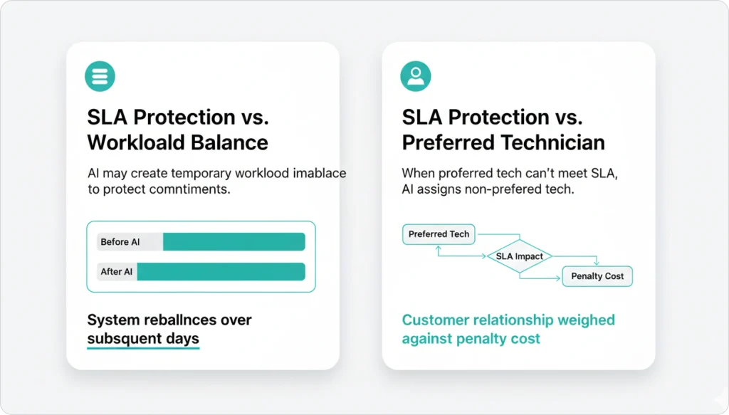
- Real-time breach-risk math runs every 5–10 minutes against GPS, traffic, and job-progress data. Above 30% risk the AI triggers protective reassignments automatically.
- Reserving 15–20% SLA shadow capacity drops violation rates by roughly 70% versus operations scheduled to 100% capacity.
- A 10-tech HVAC shop with 50 warranty jobs/week and a 5% violation rate pays $52,000–$130,000/year in penalties. Cutting violations to 1% saves $41,600–$104,000 annually.
Most shops treat SLAs the same way they treat a to-do list: deadlines written down, then hoped for. A manual dispatcher catches breaches when they’re already happening — Tech Mike is forty minutes behind, his 2 PM warranty job is at risk, and now you’re picking which of three downstream customers gets the apology call. SLA aware scheduling rewrites that workflow. The deadline isn’t a calendar event; it’s a weighted constraint inside the solver that gets heavier as the clock ticks down. The AI reassigns jobs before the breach happens, not after.
This guide explains the three SLA types every field service operation manages, the penalty escalation curve that pushes at-risk jobs to the front of the queue, the live breach-risk math that runs every 5–10 minutes, and the shadow capacity math that drops violation rates by 70%. Every formula below runs inside the live field service management software from FieldCamp.
Three Types of SLA Commitments
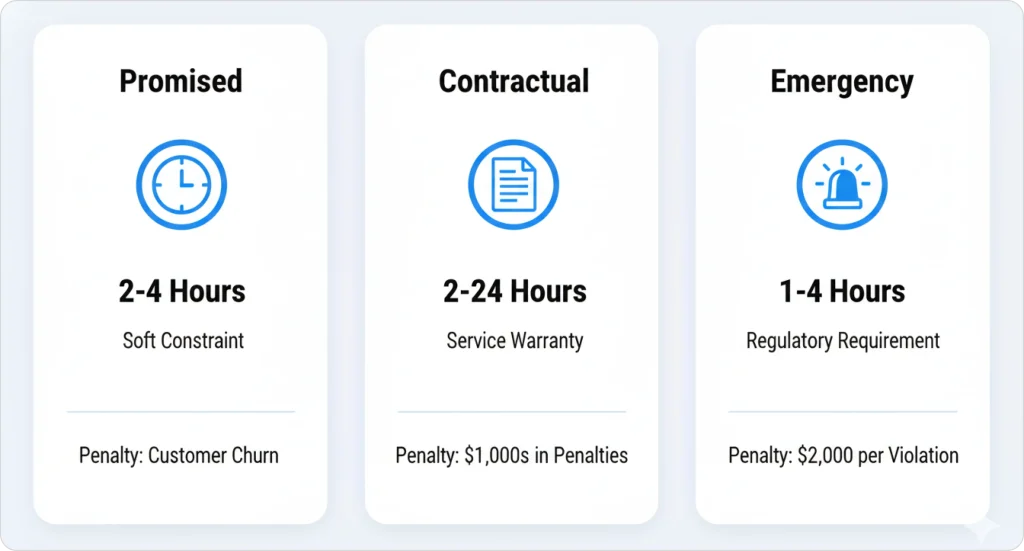
Not all service commitments carry the same weight. AI dispatch systems distinguish three types so the solver can apply the correct penalty curve to each. Mixing them up is the most common reason “we’re already tracking SLAs” projects fail in their first quarter — promised arrival windows and contractual warranty deadlines need very different penalty math.
| SLA type | Description | Typical window | Breach penalty |
|---|---|---|---|
| Promised time windows | Customer preference (soft constraint) | 2–4 hour windows | Customer dissatisfaction, potential churn |
| Contractual SLAs | Warranty / service-contract obligations | 2–24 hours | Hundreds to thousands of dollars |
| Emergency response SLAs | Regulatory / safety requirements | 1–4 hours | $300–$2,000 per violation |
Promised windows live alongside time-window optimization. Contractual SLAs are typically warranty terms tied to credits, penalties, or renewal risk. Emergency response SLAs are often regulatory and may carry the steepest per-incident cost. Categorizing SLA types lets the AI know which commitments carry contractual penalties versus customer preferences and assign penalty weights accordingly.
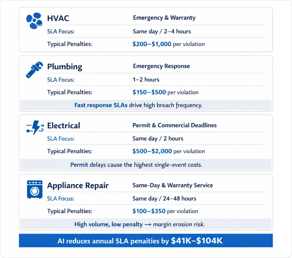
The math is unflattering. A 10-technician HVAC shop with 50 warranty jobs per week and a 5% violation rate pays roughly $52,000–$130,000 annually in penalties. Cutting violations to 1% saves $41,600–$104,000 per year. SLA-aware scheduling exists to capture that delta automatically — and the same engine powers AI dispatch scheduling across the rest of the operation.
Penalty Escalation Pushes At-Risk Jobs to the Front
Penalty escalation is the mathematical process by which the AI increases the constraint weight of an SLA commitment as its deadline approaches. A job with a 24-hour SLA window starts at a baseline weight of 100, escalates to 500 at 24 hours out, jumps to 2,000 at 4 hours out, hits 10,000 at 1 hour out, and becomes a hard constraint at 30 minutes. At the hard threshold, the AI sacrifices any other optimization goal to prevent breach.
| Time to deadline | Constraint weight | Priority level |
|---|---|---|
| Baseline (window opens) | 100 | Low |
| 24 hours before | 500 | Medium |
| 4 hours before | 2,000 | High |
| 1 hour before | 10,000 | Critical |
| 30 minutes before | HARD CONSTRAINT | Cannot be violated |
Worked example. 9:00 AM: a warranty job is scheduled for 2:00 PM. Weight 100, low priority. 12:00 PM: the tech is running 45 minutes late on his previous job. Weight jumps to 500, medium priority. 1:00 PM: breach risk now 60%, weight escalates to 2,000, AI reassigns two downstream jobs. 1:30 PM: breach risk 85%, weight hits 10,000, AI pulls the nearest available tech even if it breaks the route. When SLA constraint weight exceeds 2,000, the AI accepts up to a 25% increase in total drive time to prevent a violation. A 25% drive-time increase costs roughly $12 in fuel and labor — acceptable when avoiding a $500 penalty.
This escalation is one of the strongest signals that pushes a job to the front of the queue inside job-to-technician matching. The system isn’t running a separate “SLA module” — it’s adjusting the cost function the route optimizer already uses.
KEY TAKEAWAY
Manual dispatch protects SLAs in retrospect — Mike’s at-risk warranty becomes a problem at 1:30 PM. AI protects SLAs in advance: by 12 PM the weight has already climbed to 500 and the schedule starts adjusting around it. Same data, different math, very different outcome.
Real-Time Breach Risk Math

Breach risk is the live probability that a given SLA commitment will be missed given current conditions. AI dispatching calculates breach risk every 5–10 minutes, triggering protective actions when risk exceeds 30%. The system tracks job progress and estimated completion time, GPS coordinates (updated every 1–5 minutes), live traffic conditions, and historical job-duration patterns.
Formula. Breach Risk = (Time remaining to SLA deadline) − (Estimated time to complete current job + drive time to SLA job).
When breach risk crosses threshold, the AI triggers protective reassignments through the same AI route optimization engine that handles standard routing — there’s no parallel system to keep in sync.
| Breach risk | Action |
|---|---|
| < 30% | Standard route optimization |
| 30–50% | Minor route adjustments accepted |
| 50–70% | Significant rerouting, possible reassignment |
| > 70% | Full reassignment, efficiency secondary |
| > 90% | Hard constraint — any available tech dispatched |
Worked example. Technician Mike is 30 minutes into a 90-minute HVAC install with three remaining warranty jobs, all on 4-hour SLAs. At 10:15 AM traffic spikes on his route. The AI calculates: Job 1 breach risk 15% (safe), Job 2 45% (warning), Job 3 72% (critical). Job 3 reassigns to Sarah, who’s 12 minutes farther but has open capacity. Mike’s route gets 8 minutes longer; all SLAs are protected.
Cascading impact. One delay can put 3–8 downstream SLAs at risk. The AI ranks which SLAs to protect based on penalty cost (higher penalties get priority), customer tier (VIP, premium), and contract value ($50K annual contract vs. one-time service call). When breach risk exceeds 50%, the AI accepts up to a 30% route-efficiency loss to prevent the violation. A 10-minute detour costing $4 in fuel is worth it to avoid a $400 SLA penalty.
PRO TIP
Use the labor cost calculator to map your team’s hourly cost against your SLA penalty schedule. The trade-off math is more profitable than most dispatchers realize — $12 in extra labor protects a $500 penalty every time.
Cut SLA Violations by 70%
Run your warranty workload through the FieldCamp AI Dispatcher. We’ll model penalty savings against your real volume in a 30-minute demo.
SLA Shadow Capacity Drops Violations 70%
SLA shadow capacity is the portion of daily scheduling capacity (typically 15–20%) reserved as buffer for SLA-protected jobs that may need emergency rescheduling due to technician delays, traffic, or job overruns. For a 10-technician team completing 80 jobs/day, shadow capacity means initial planning schedules only 64–68 jobs and holds 12–16 slots open to absorb SLA-related disruptions.
Operations that reserve 15–20% shadow capacity experience roughly 70% fewer violations than operations scheduled to 100% capacity. The math is brutal and obvious: a fully-booked schedule has no headroom to protect anything when one job runs long.
Maximum SLA-protected jobs = Technician count × Average jobs per day × SLA buffer percentage.
Buffer guidelines: 15–20% for high-reliability operations, 25–30% for variable job durations or unpredictable service areas. A 5-tech plumbing company averaging 6 jobs/tech/day (30 total) with 20% shadow capacity = 24 SLA-protected jobs/day max. If they accept 28 SLA commitments, breach risk jumps from 2% to 12%, costing roughly $18,000 annually in penalties.
| SLA type | Acceptable breach risk | Action threshold |
|---|---|---|
| Contractual | 1–3% | Immediate escalation at 2% |
| Promised time windows | 5–8% | Review at 6% |
| Emergency response | < 1% | Zero tolerance policy |
The buffer rules feed directly into broader headcount and overflow math through capacity planning with AI. When the issue is unscheduled urgent work rather than steady SLA demand, the same engine routes those through emergency job handling without competing for the SLA buffer.
Industry SLA Patterns and Tracking Metrics
SLA windows and penalties vary sharply by trade. The AI doesn’t need to be told these — they’re configured once and applied automatically per job type — but the operator setting up the system needs to map them honestly.
- HVAC. Warranty 2–4 hr ($200–$500 penalty), no-heat/no-cool same-day ($300–$1,000), commercial contracts 4–8 hr ($400–$800).
- Plumbing. Emergency 1–2 hr ($150–$300), warranty same-day ($200–$400), commercial 2–4 hr ($250–$500).
- Electrical. Permit deadlines same-day ($500–$2,000 — often the most expensive SLA violations in field service), commercial 2-hr response ($400–$800), residential 4-hr ($200–$400).
- Appliance repair. Same-day commitments ($100–$250), warranty manufacturer requirements 24–48 hr ($150–$350).
Five metrics tell you whether the system is doing its job. SLA Violation Rate (target < 2%, violations ÷ total SLA jobs). Average Breach Risk (target < 20%, mean across all SLA jobs). Shadow Capacity Utilization (60–80%, buffer slots used ÷ reserved). Penalty Cost per Month (trending down). Reassignment Rate (5–10%, jobs reassigned for SLA protection).
WARNING
If reassignment rate exceeds 15%, the operation is over-scheduling SLA commitments relative to capacity. Reduce new bookings or add technician headcount. Pumping more jobs into the schedule with the assumption “AI will sort it” guarantees burn-out and breach.
For a sanity check on whether you’re pricing SLA work correctly, the HVAC pricing guide walks through warranty job margins by region.
How FieldCamp Protects SLA Commitments

FieldCamp’s SLA protection runs the penalty escalation formula (100 → 500 → 2,000 → 10,000 → HARD) to automatically prioritize at-risk commitments. The system reserves 15–20% shadow capacity, recalculates breach risk every 5–10 minutes, and triggers protective reassignments when risk crosses 30%. No dispatcher intervention required.
Real-time monitoring inside the AI Command Center tracks job progress, GPS coordinates, traffic conditions, and historical patterns. When delays hit, the escalation curve handles protection automatically. Compared with manual SLA tracking that treats deadlines as static, the system identifies affected downstream jobs, calculates new arrival times, decides which SLAs to protect, makes reassignments, and notifies affected customers — every 5–10 minutes, across the entire operation.
Set this up in the docs:
Behind the scenes, the same constraint solver that handles SLA escalation also powers work order management, so warranty terms stay tied to the work order they originated from. Mid-job rescheduling routes through the same continuous planning endpoint that handles normal dispatch — there are no parallel SLA workflows to maintain.
Stop Paying SLA Penalties
FieldCamp’s AI Dispatcher escalates at-risk warranty jobs automatically and reassigns before the breach happens. See it run against your real schedule.
Frequently Asked Questions
What is SLA aware scheduling?
SLA aware scheduling treats service-level agreement deadlines as weighted constraints inside the dispatch solver. As the risk of missing a deadline rises, the AI increases that job’s constraint weight so it overrides goals like shortest travel time or workload balance — protecting contractual commitments first.
How does penalty escalation work?
A job’s constraint weight starts low when the SLA window opens and escalates as the deadline approaches: 100 to 500 at 24 hours out, to 2,000 at 4 hours out, to 10,000 at 1 hour out, and becomes a hard constraint at 30 minutes. At the hard threshold the AI sacrifices any other optimization goal to prevent breach.
What is SLA shadow capacity?
SLA shadow capacity is the 15 to 20 percent of daily scheduling capacity reserved as buffer for SLA-protected jobs that may need emergency rescheduling. Operations that hold shadow capacity experience roughly 70 percent fewer violations than operations scheduled to 100 percent capacity.
How often does the AI check breach risk?
Every 5 to 10 minutes during active jobs. The system processes traffic, GPS location, and job-status updates in real time, triggering protective reassignments when breach risk exceeds 30 percent.
Will the AI break a route to save an SLA?
Yes, when the math justifies it. When breach risk exceeds 50 percent the AI accepts up to a 30 percent route-efficiency loss to prevent the violation — a $4 fuel detour to avoid a $400 SLA penalty is a clear trade-off the algorithm makes automatically.
How does SLA aware scheduling differ from emergency dispatch?
SLA aware scheduling protects pre-existing commitments as their deadlines approach. Emergency dispatch handles unscheduled high-priority calls that arrive mid-day. The two systems share the constraint solver but trigger on different signals.
Continue reading
- Time window optimization — how promised windows feed into SLA penalty curves.
- Emergency job handling — what to do when SLA pressure becomes a P0 call.
- Dynamic rerouting — the runtime engine that protective reassignments call into.
- AI dispatcher ROI calculator — model penalty savings against your real warranty volume.